Writing this post was kind of depressing, because all it did was highlight for me how many things I’ve got in my reading list to think about and digest. I was reading Brad DeLong’s recent post on manufacturing’s share in output, and realized that I’ve got about four more posts from Brad stacked up in the queue, along with all the other stuff I’ve been meaning to read more carefully. So, respectfully, Brad, please stop saying interesting things related to growth. I need time to catch up. How about a nice run of posts about the history of monetary policy or something like that?
DeLong’s motivating fact(s) are about manufacturing’s share of output, both in nominal and real terms. He grabbed the following from the BEA
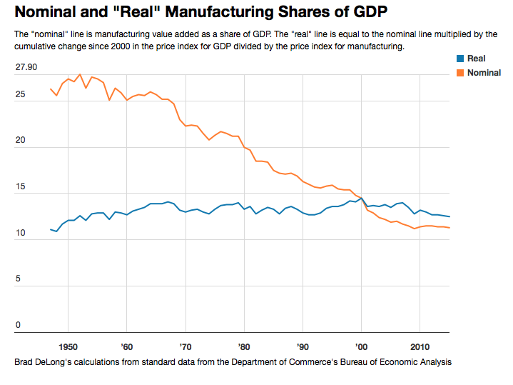
and developed the path of the real share by making a crude calculation. As he freely admits in the post, this isn’t exactly how one would want to calculate the real share of manufacturing in output. But, for the purposes of his post, I don’t think it makes a huge difference.
Anyway, he establishes three main facts that he wants to understand. First, note that the nominal share of manufacturing in nominal output has been declining steadily since the late 1940’s. He gets a value of -1.4% per year as the growth rate of the nominal share. Second, the relative price of manufactured goods (compared to aggregate output) has been declining by -1.4% per year as well. This gives us the final fact, that the real share of manufacturing in real output has not grown (or shrunk) over time, as you can see in the figure.
DeLong then proceeds to ask himself how to reconcile all of these three facts. What must be true about demand and/or technological change to explain this? And he will come to a conclusion that we are probably not measuing the price decline, and hence the real share of manufacturing, correctly. That will in turn imply that real economic growth has probably been understated over this entire period of time.
I think DeLong is too quick to make that conclusion, and that there is in fact a way to understand his three facts that does not imply economic growth has been understated. My brain moves a little slower than DeLong’s, so here’s how I worked through his reasoning. First, let the following be the demand curve for real manufacturing goods, in log terms
\[\ln Q^M = \epsilon_I \ln Y - \epsilon_P \ln P^M + \ln D^M\]where $Q^M$ is the quantity of real manufactured goods, $Y$ is real income, and $P^M$ is the relative price of manufactured goods. $\epsilon_I$ is the income elasticity of demand for manufactured goods, and $\epsilon_P$ the price elasticity of demand. $D$ is just a “demand shifter” to account for anything changing demand for manufactured goods that isn’t related to either real income or the relative price.
Add $\ln P^M$ to both sides, and subtract $\ln Y$ from both sides. That leaves me with
\[\ln Q^M + \ln P^M - \ln Y = (\epsilon_I-1) \ln Y + (1 - \epsilon_P) \ln P^M + \ln D^M.\]The left-hand side is, if you combine the log terms, $\ln Q^M P^M/Y$, or the log of manufacturing’s share in nominal income. Also, it’s important to note that the left-hand side can be written as $\ln Q^M/Y + \ln P^M$. This is the log of manufacturing’s share of real income, plus the relative price level of manufactured goods. So it has both the nominal and real share of manufacturing in it.
To work with this in DeLong’s terms, it will be easiest to talk about growth rates of all of these items. And with everything written in log terms, getting growth rates is straightforward. Let $\hat{q}^M$ indicate the growth rate of real manufacturing goods, and define a similar “hat” term for each element of the equation. We’ve got
\[(\hat{q}^M - \hat{y}) + \hat{p}^M = (\epsilon_I-1) \hat{y} + (1 - \epsilon_P) \hat{p}^M + \hat{d}^M.\]Notice that I’ve done a little rearranging there. Inside the parentheses on the left is the growth rate of manufacturing’s real share of real income. That gets added to the growth rate of the relative price of manufacturing to deliver the growth rate of manufacturing’s share of nominal income.
Let’s go back to DeLong’s pieces of information. First, the growth rate of the nominal share of manufacturing is -1.4% per year. This means that $(\hat{q}^M - \hat{y}) + \hat{p}^M = -0.014$. Second, he says that the growth rate of the relative price of manufactured goods is also -1.4% per year, meaning that $\hat{p}^M = -0.014$. Last, the data said that the growth rate of the manufacturing’s real share of real output was zero, meaning that $(\hat{q}^M - \hat{y}) = 0$.
Then he goes to work trying to understand how all of those facts can be true at the same time, given the above equation. Here are two possibilities that DeLong dismisses as not making sense - and I think he’s right to dismiss these possibilities.
-
If the income elasticity is 1 and the price elasticity is 1, then $(\hat{q}^M - \hat{y}) + \hat{p}^M = \hat{d}^M$. Which means that $0 + -0.014 = \hat{d}^M$. In other words, there must have been a sustained shift in the demand curve for manufactured goods over the last 70 years. We just decided we didn’t like manufactured stuff as much any more. DeLong says this doesn’t make sense. That’s probably right, but hold onto that thought about a shift in the demand for manufactured goods - it will show up again later in the post.
-
If the income elasticity is 1 and the price elasticity is 0, then $(\hat{q}^M - \hat{y}) + \hat{p}^M = \hat{p}^M + \hat{d}^M$. Then, plugging in the facts, we have that $\hat{d}^M = 0$. DeLong says this helps, because it doesn’t require us to assume any kind of exogenous shift in demand for manufactured goods. But, it does require us to assume that the price elasticity is zero, which DeLong says doesn’t make sense because manufactured stuff is useful, so you’d expect that demand would go up if the price fell. That’s probably right, too - the price elasticity probably isn’t zero.
DeLong then asks how this is all supposed to work if we instead assume that the income elasticity is 1, the price elasticity is something more reasonable like 1/2, and we dismiss the idea of a purely exogenous shift in manufacturing demand. And this leads him to a problem with reconciling the data. With those assumptions, it means that the growth rate equation is
\[(\hat{q}^M - \hat{y}) + \hat{p}^M = 0.5 \hat{p}^M.\]In this equation, it is impossible for DeLong’s facts to all be true simultaneously. That is, we can’t have the growth rate of the real share (in the parentheses) be zero, the growth rate of the nominal share (the entire left-hand side) be equal to -0.014, while at the same time $\hat{p}^M = -0.014$ on the right-hand side.
How to fix this? DeLong suggests that both his second and third facts are probably wrong. If the relative price of manufacturing actually fell by 2.8% per year, so $\hat{p}^M = -0.028$, and the real share of manufacturing actually grew by 1.4% a year, so $(\hat{q}^M - \hat{y}) = 0.014$, then everything works out. Specifically, $0.014 + -0.028 = 0.5\times-0.028$.
So if we assume a reasonable price elasticity of 1/2, and if we take the growth rate of the nominal share of manufacturing (which is relatively easy to measure) as given, then we cannot do anything but conclude that the growth rate of the real share of manufacturing was in fact 1.4% per year, not zero. Over the roughly 70 years DeLong is talking about, that means the real share of manufacturing should be about 2.5 times higher than we observe in his graph. It would be about 28% of real output today, not 12%.
With the relative price of manufacturing falling twice as fast as we thought, and real manufacturing output growing relative to real output, this implies that we really are better off than we thought. I won’t get into the mechanics of this calculation here, as the post is already getting long, but it would imply that real output growth was actually about 0.3 percentage points higher per year over this period. Real output grew at about 3 percent per year, so that’s a pretty big difference.
But here is where I think DeLong’s gone one step too far. He focuses on the price elasticity, but assumes the income elasticity is equal to one in all cases. His alternative scenario where growth in the real manufacturing share and faster true growth in real output is contingent on this assumption. Let me propose an alternative way of reconciling the numbers that doesn’t imply anything is mismeasured.
Let’s use DeLong’s price elasticity of 1/2. I don’t have any strong reason to quibble with that number. And let’s retain the assumption that there is no exogenous demand shift. But rather than assuming the income elasticity is one, let’s leave it as a free variable. So now the growth rate equation is
\[(\hat{q}^M - \hat{y}) + \hat{p}^M = (\epsilon_I-1) \hat{y} + 0.5 \hat{p}^M.\]Take the original facts as correct, and let me add one additional fact. The growth rate of real income reported by the BEA over the same time period as DeLong is working with is 3% per year. This is the growth rate of aggregate real income, not per capita. Putting all this in our equation gives me
\[0 + -0.014 = (\epsilon_I-1) 0.03 + 0.5 \times -0.014\]and everything makes sense if $\epsilon_I = 0.77$. That is, if the income elasticity of demand for manufactured goods is a little less than one. An elasticity less than one means that if your income goes up by 10%, your expenditure on manufactured goods rises by less than 10%. It goes up, but not by a similar percent. This income elasticity less than one acts a lot like the “demand shift” that DeLong dismisses in his first scenario. If you like, I’ve just given a very specific form to that demand shift.
Is that reasonable? I sure think it is. It’s entirely consistent with the literature on structural change for rich countries like the US. Income elasticities for manufacturing less than one reflect people’s preferences having some kind of “limit” on the amount of manufactured goods they want to consume. I’ve used the refrigerator example before. If we get even more productive at producing refrigerators, then they will become less costly and/or become higher quality. But that doesn’t mean I’ll buy another one. I’ve got two at my house already, and it would take a massive drop in price or increase in quality to get me to buy another one, even just to replace the existing ones. Similarly, my income is due to go up in October thanks to the raise pool at UH this year. I’m not using it to buy a fridge, or probably many manufactured goods at all. I’ll use it to help pay for a trip we’re taking in December.
So the original facts that DeLong lays out are entirely consistent, including the fact that the real share of manufacturing in output has stayed constant over time. We don’t need to assume that prices fell faster than we thought, or that real manufacturing output grew faster than we thought. And thus output growth isn’t understated.
DeLong could still be right, of course. This is all dependent on competing assumptions about the size of elasticities. If the income elasticity is actually one, then DeLong’s story is more plausible than mine. I think I’m on the right track, but I don’t have the time at the moment to collect various references to back up my income elasticity argument.
One last interesting note. The income elasticity doesn’t have to be constant over time. In fact, I’d guess it was closer to one, if not higher than one, back in the early part of the period DeLong considers, the 1940’s and 1950’s. If the income elasticity is bigger than one, then this means DeLong’s adjustments for that period would be even bigger than what he calculated in his post. I have to think harder about this, but I’m wondering if this is some way to reconcile/explain Robert Gordon’s facts about rapid measured productivity growth in those decades relative to the current period of time. Stay tuned.