Dev Patel, Justin Sandefur, and Arvind Subramanian posted the other day some new evidence on cross-country convergence. They showed that there is statisticaly significant evidence for unconditional convergence in GDP per capita across countries. I’ll get to more details below, but in short they find that poor countries grow faster than rich ones, on average.
They set this up as a counter-point to an article coming out in the Journal of Economic Literature by Paul Johnson and Chris Papageorgiou that says cross-country convergence doesn’t occur. The difference in the PSS post and the JP paper is that PSS look at relatively recent windows of data. For example, PSS look at whether countries that were poor in 1990 grew faster than rich countries in 1990 from 1990 to 2014.
In constrast, JP appear to look at longer time frames. They find that there isn’t much evidence countries that were poor in 1960 grew faster than rich countries in 1960. This isn’t a contradiction with PSS. Both can be true at once. All PSS have done is indicated that around twenty-five years ago poor countries did start growing faster than rich countries.
The implication of that finding is that poor countries are converging to rich country GDP per capita. And while that statement is defensible, it does need a host of qualifications, because it doesn’t mean you should expect that developing countries are soon going to look like Western Europe. This post is meant to pick through those qualifications.
Flavors of convergence
Let’s start with a better definition of convergence. There are two kinds. Within economics, they acquired particular names, and I’ll use those to be consistent with the literature. They are:
-
$\beta$-convergence: this kind of convergence occurs if the growth rate of GDP per capita is negatively related to the initial level of GDP per capita. That is, $\beta$-convergence is defined by poor countries growing faster than rich countries.
-
$\sigma$-convergence: this kind of convergence occurs if the variance (or any measure of dispersion, really) of GDP per capita across countries shrinks. $\sigma$-convergence means the gap in GDP per capita from rich to poor gets smaller.
Now, it feels like $\beta$-convergence should imply $\sigma$-convergence. And in some cases it does. Rather than GDP per capita, think about the height of the people in my house. If you plotted the growth rate of height from 2005-2018 against height in 2005 for all four of us, you’d get a negative coefficient. My two daughters were really short in 2005, but grew very fast over the next 13 years. My wife and I were both relatively tall in 2005, but neither of us grew at all. That’s $\beta$-convergence. In this case, if you looked at the variance of heights in 2005, that would be much larger than the variance of heights in 2018, and hence there was also $\sigma$-convergence in my house.
For height, $\beta$-convergence implies $\sigma$-convergence because there is not any additional noise or variance in height to worry about. I don’t wake up every day and randomly find myself 6 inches taller or shorter than I was the day before. That ensures that as my daughters grow, they really do catch up in height. I don’t get randomly taller, and they don’t get randomly shorter.
But in the case of economic growth, there are random shocks to GDP per capita. $\beta$-convergence says that poor countries, on average, grow faster than rich countries. But there will be instances where poor countries have really slow, or negative, growth sometimes. Think of currency crises or political upheavals. There will be some instances where rich countries experience rapid growth. With both of these things going on, it’s entirely possible that poor countries keep falling farther behind in terms of GDP per capita, $\sigma$-divergence, even though the poorer they get the faster they grow on average.
Here’s an analogy that could help. Imagine somone one juggling bowling pins. Gravity is like$\beta$-convergence. If the bowling pin is up in the air, then gravity is making it fall. But every time it reaches the juggler, she throws it back up in the air. This means there is always the same amount of dispersion in the location of the pins; some are up and some are down. In other words, there is a constant amount of $\sigma$-convergence, even though the $\beta$-convergence caused by gravity is always at work. If the juggler throws the pins up with a little less force each time, then the dispersion will decrease. If the juggler throws the pins up with more force each time, the dispersion will increase. Nevertheless, gravity - $\beta$-convergence - is still working the whole time.
Economic shocks act a little like the juggler, except that it isn’t just the rich countries (the ones the juggler catches) that experience shocks (the toss in the air). But the principle is similar, which is that with sufficiently large shocks, the dispersion in GDP per capita may not fall, and could even rise, over time. This is true even though $\beta$-convergence, like gravity, operates on countries the whole time.
In terms of cross-country comparisons, we’re mainly interested in $\sigma$-convergence: is the gap between poor and rich countries shrinking over time? Observing $\beta$-convergence in the data does not tell us whether that is true. Now, some sort of $\beta$-convergence is necessary for $\sigma$-convergence to occur. At some point, a poor country has to grow faster than a rich country in order to catch up. But $\beta$-convergence isn’t sufficient for $\sigma$-convergence. The PSS result doesn’t mean that the dispersion of GDP per capita across countries got smaller, or will get smaller.
Convergence speed
Let’s leave aside whether $\beta$-convergence implies $\sigma$-convergence for the moment. Let’s assume that the shocks are small enough that in fact, $\sigma$-convergence is implied. The next question is how long it will take a poor country to close the gap with a rich country, and the actual coefficient that PSS estimate can tell us about this.
To make sense of this, I need a little math. The convergence relationship that PSS estimate looks like this
\[\frac{\ln y_{t} - \ln y_0}{t} = \alpha + \beta \ln y_0.\]On the left is the growth rate of GDP per capita, $y$, from some initial year 0 to year $t$. This is related to the initial level of GDP per capita, $y_0$, on the right-hand side. The strength of that relationship is measured by the coefficient $\beta$. $\beta$-convergence means that $\beta<0$, or that the growth rate gets smaller as the initial level of income gets higher. How large (in absolute value) $\beta$ is determines how strong that effect is. The extra parameter $\alpha$ is a baseline growth rate.
A little re-arrangment of this gives us
\[\ln y_t = \alpha t + (1 + \beta t) \ln y_0\]which is the level of GDP per capita at time $t$, given initial GDP per capita at time 0. That multiplicative term $\beta t$ is the effect of $\beta$-convergence over time.
Using this, here’s a question we could ask. Given a poor country has $y_0^{Poor}$ that is only 10% of the value in a rich country, $y_0^{Rich}$, how long will it take (i.e. how big does $t$ have to be) before $y_t^{Poor}$ is 90% of the value in the rich country, $y_t^{Rich}$? Given the set-up, this will happen at some point. I didn’t add any of the shocks mentioned above that could keep spreading these two countries apart. $\beta$-convergence will eventually win out.
At this hypothetical time $t$, we want that $y_t^{Poor}/y_t^{Rich} = .9$, which if you take logs and plug in from the above equation, gives us
\[\ln .9 = \alpha t + (1 + \beta t) \ln y_0^{Poor} - \alpha t - (1 + \beta t) \ln y_0^{Rich}\]and we can simplify this to
\[\ln .9 = (1 + \beta t) (\ln y_0^{Poor} - \ln y_0^{Rich}).\]We also said that $y_0^{Poor}/y_0^{Rich} = .1$, so taking logs of that, we can plug in and get
\[\ln .9 = (1 + \beta t) \ln .1\]and now re-arrange to solve for time $t$
\[t = \frac{\frac{\ln .9}{\ln .1} - 1}{\beta}.\]This is how long it will take the poor country to go from 10% of rich country GDP per capita to 90% per capita. And you could plug in other numbers in the obvious spots here to think about the time to go from 20% to 99%, or whatever you wanted.
The key is that the absolute size of $\beta$ matters. The smaller is $\beta$ in absolute value, the more time it takes to converge. Now, what PSS show is that in samples that only run through 2000, $\beta$ was about 0, which means that $t$ is essentially infinity. With no $\beta$-convergence, there isn’t a way for the poor country to ever catch up, because it doesn’t grow faster than the rich country. But with later samples, $\beta<0$, so they can.
Their biggest estimate value is $\beta = -.005$, not very big. Plugging that into the above equation implies that $t = 190$, or it will take about 190 years for a country to go from 10% of rich-country GDP per capita to 90%. That’s a loooong time. So even in the case where we assume that $\beta$-convergence leads to $\sigma$-convergence (i.e. the ratio goes from 10% to 90%), and ignore the possibility that shocks keep spreading things out, $\beta$-convergence may not imply much noticeable $\sigma$-convergence over the next few decades.
Absolute and conditional convergence
The PSS result of $\beta = -.005$ is small. At the same time, you will see references that the convergence coefficient is more like $\beta = -0.02$ in the literature. Probably the most famous of these papers are from Barro in 1991 and Barro and Sala-i-Martin in 1992. There are a host of other papers offering more estimates of this parameter, but I think it is fair to say that -0.02 is a good eyeball average of those results.
Now, we have to be a little careful here in these older results to PSS. PSS estimate unconditional $\beta$-convergence, meaning they just making raw comparisons of growth in GDP per capita against initial GDP per capita across countries. Their result implies that poorer countries grow (a little bit) faster than rich countries, and that this doesn’t depend (is unconditional) on characteristics of those countries. It says that if you are poor, no matter why you are poor, you grow a little faster than rich countries, no matter why they are rich.
The original convergence literature did the same kind of unconditional analysis, and found nothing. That is the point, in some sense, of the PSS note. But that original literature did find evidence for conditional $\beta$-convergence. This means that if you look only at groups of countries that have similar characteristics (e.g. savings rate, human capital levels, etc..) then you find $\beta$-convergence in those groups - the poorer ones grow faster than the rich ones.
But across groups, there was no tendency for $\beta$-convergence. For example, if you looked only at the OECD countries, you’d see pretty strong evidence of $\beta$-convergence, with an estimate of $\beta = -0.02$, roughly. And if you looked only at the set of Sub-Saharan African countries, you’d see similar evidence of $\beta$-convergence. But, there was no tendency for SSA countries as a group to grow faster than OECD countries. It was only that within the group of SSA countries, poorer ones grew faster, and within the group of OECD countries, poorer ones grew faster. You can find this notion of conditional - or “club” - convergence in blog-favorite William Baumol’s 1986 paper that was one of the first to think about this topic.
A different way of looking at conditional convergence was to use data on states or prefectures within a single country. They would all have roughly similar characteristics relative to countries (e.g. Texas and Florida differ, but that difference pales in comparison to the difference between Texas and Nigeria). And within countries, the evidence seems was clear that $\beta$-convergence happens. Again, these coefficients were usually around $\beta = -0.02$.
The $\beta = -0.02$ number implies much faster convergence. If you think of a poor state that had 10% GDP per capita relative to a rich state, then it would only take about 48 years for it to reach 90% of GDP per capita of the rich state. That’s, not surprisingly, one-fourth the time it takes a poor country to catch up to a rich one. It’s also one way of thinking about why we don’t see U.S. states with only 10% the GDP per capita of rich ones. Any time a gap opens up, it tends to dissipate. Although I need to note that there is some recent research saying that $\beta$-convergence across U.S. states no longer occurs. Let’s leave that aside.
Which number is right, $\beta=-0.005$ or $\beta = -0.02$? Neither. They don’t measure the same thing. The former is for unconditional cross-country convergence in the last 25 years, the latter is appropriate for conditional convergence or within-country convergence. Both can be true in their individual setting. Individual provinces within Kenya might converge very quickly, even though Kenya as a whole isn’t converging very quickly to U.S. GDP per capita.
What does convergence tell us?
The use of convergence results depends on what you’re after. The $\beta$ value that PSS report, similar to every other estimated $\beta$ value, tells you whether on average poor countries grow faster than rich ones. But that doesn’t make it very informative about any particular country. It certainly won’t tell you whether to expect some kind of growth miracle or disaster to occur in the future.
Here’s what I mean. I took the Penn World Tables, one of the datasets used by PSS, and plotted the data used to estimate $\beta$. You’ve got the average growth rate of GDP per capita from 1990 to 2014 on the y-axis, against the (log) of GDP per capita in 1990 on the x-axis. The downward-sloped dashed line is the best fit to this data, and the slope of that line is about -.005, the PSS estimate of $\beta$.
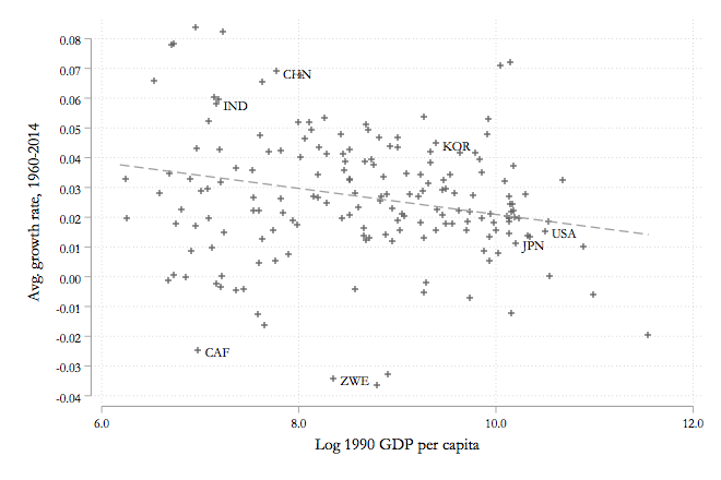
But you can see that this hides a lot of variation. I labelled a few countries for reference. The USA and Japan (JPN), out on the right, can be the stand-in for the “Rich” countries. You can also see China (CHN) and India (IND), both of which had growth rates well above the estimated relationship, and hence they converged much faster towards rich-country GDP per capita. This would set them apart from the Central African Republic (CAF) and Zimbabwe (ZWE), who both started out relatively poor, but shrank in terms of GDP per capita, and fell even further behind the USA and JPN. I also threw South Korea (KOR) in there, as an example of a country that closed almost the entire gap with JPN from 1990 to 2014, although many other countries with a similar level of GDP per capita in 1990 did not.
A crude way of seeing how useful the $\beta$-convergence result is comes from looking at the R-squared of the regression that was used to estimate $\beta$. It’s 0.0462. In other words, 95.38% of the variation in growth rates from 1990 to 2014 is not explained by how poor a country was in 1990. Yes, there is evidence here for unconditional convergence on average. But plenty of countries grew slower than necessary to converge to rich country levels of GDP per capita.
It is probably best not to think of unconditional $\beta$-convergence as representing some kind of structural truth about economic growth. If it were, you’d expect it to show up regardless of the exact time frame looked at, and PSS show that’s not the case. It’s better to think of it as a summary statistic of the general experience of poor countries in a given time frame. The PSS results tell us that something changed around 1990 such that many poor countries grew faster than rich countries, relative to the period from 1960 to 1990. But it doesn’t tell us what or why it changed, or if it will persist.
That doesn’t make the PSS estimate spurious. It’s a nice descriptive result that tells us we should think a little more about what might have changed around those years, even if the implication of $\beta$-convergence from that period is not that strong.