There was a recent post by an engineer rebutting Robert Gordon’s (and others) thesis that technological change was slowing down. The evidence cited is a series of plots and figures showing how specific technologies (battery storage, energy efficiency, computer speed, etc..) are advancing just as fast as they have for decades, if not faster. And there were a number of responses along the lines of “See, Gordon is wrong!”.
The mistake here is that this doesn’t constitute evidence that Gordon is wrong. But the mistake is partly forgivable because Gordon himself indulges in these kinds of anecdotal arguments to advance his thesis, and so it seems as if you could refute his conclusions by offereing alternative anecdotes.
But the important part of Gordon’s argument is not that specific technologies are or are not advancing. It is that aggregate productivity growth is slowing down. And aggregate productivity growth depends not only on individual technologies, but crucially on the distribution of workers using those technologies. Arguing about only those individual technologies is like using an increase in the price of milk to argue that inflation must be high.
Aggregate productivity growth depends on what we can call “within-sector” growth, which is going to be tied closely to those individual technologies. But it also depends on “across-sector” growth, which is tied to the movement of workers from one sector (or job) to another. If workers are shifting from high- to low-productivity sectors or jobs, then aggregate productivity growth may fall even though nothing happened to actual technological change.
I’ll make this more clear below, but here’s a quick summary of what I’ll try to establish. Gordon’s critics could well be right about their individual technologies, and yet wrong about this having anything to do with aggregate growth, because those sectors may not employ many people. And Gordon can be right about aggregate growth, but wrong about individual technologies stagnating, because the movement of workers to low-productivity sectors may be dragging down growth. In short, you cannot talk about aggregate productivity growth without talking about both technology and the distribution of workers across sectors.
Gruesome Detail
Yes, there is math. Gordon’s argument is about the growth rate of total factor productivity (TFP). But sector and industry level data on TFP isn’t available for the time frames I want, so I’m going to look instead at value-added per hour, a measure of labor productivity. TFP and value-added per hour are going to be highly correlated, but not perfectly.
Value-added per hour, $y$, is the summation across all $J$ sectors of the economy
\[y = \sum_{j=1}^J s_j y_j\]where $s_j$ is the share of total hours worked in sector $j$, and $y_j$ is the value-added per hour in sector $j$. With that definition, the change in value-added per hour from time 0 to time $t$ can be written as
\[\Delta y_t = \sum_{j=1}^J s_{jt} y_{jt} - \sum_{j=1}^J s_{j0} y_{j0}.\]This isn’t very informative by itself, but by rearranging the terms in those two summations, adding and subtracting some other common terms, and a little algebra, we can get
\[\Delta y_t = \sum_{j=1}^J \Delta y_{jt} s_{j0} + \sum_{j=1}^J \Delta s_{jt} y_{j0} + \sum_{j=1}^J \Delta y_{jt} \Delta s_{jt}.\]A couple of notes on this equation. First, this is the absolute change in value-added per hour. This isn’t the growth rate. You could divide by sides by $y_0$ to get a growth rate, but as written the equation looks simpler. Second, I’ve made precisely zero assumptions about behavior to get this. This is pure accounting.
The three separate summations on the right-hand side can be nicely interpreted.
-
Within-sector growth: $\sum_{j=1}^J \Delta y_{jt} s_{j0}$ holds constant the allocation of hours seen at time zero. This is the growth we’d get if all that happened was that each sector got more productive, $\Delta y_{jt}$, but we did not allow anyone to change jobs. The idea is to measure just improvements in labor productivity within sectors.
-
Across-sector growth: $\sum_{j=1}^J \Delta s_{jt} y_{j0}$ holds constant the value-added per hour seen at time zero. This is the growth we’d get if all that happened was that workers (and their hours of work) moved between jobs. Note that this will be positive if people move from low- to high-productivity jobs, or negative if they move from high- to low-.
-
Covariance: $\sum_{j=1}^J \Delta y_{jt} \Delta s_{jt}$ captures the fact that not only do sectors vary in their time-zero level of productivity, but differ in their productivity growth. This term captures whether or not people are moving into sectors where productivity is growing, which would show up as a positive value. A negative means that workers are moving to sectors where productivity is shrinking.
To illustrate the role of these three effects, I pulled down sector-level data from the Groningen 10-sector database for the U.S., from 1950-2010. The 10 sectors are broad - agriculture, manufacturing, construction, etc. - but have the advantage of spanning a long time frame. I can pull data from the BLS at a much finer industry level at the cost of only going back to 1987. From what I found, the BLS data confirm the story I’ll tell with the Groningen data, so let’s stick with that.
In each year, I calculated the three terms in the above equation, looking backward 10 years each time. So I have the rolling 10-year growth in value-added per hour (VAPH), as well as how it breaks down into within, across, and covariance terms. What I’ve plotted below is the total growth rate, not an annualized rate, so that everything still adds up exactly.
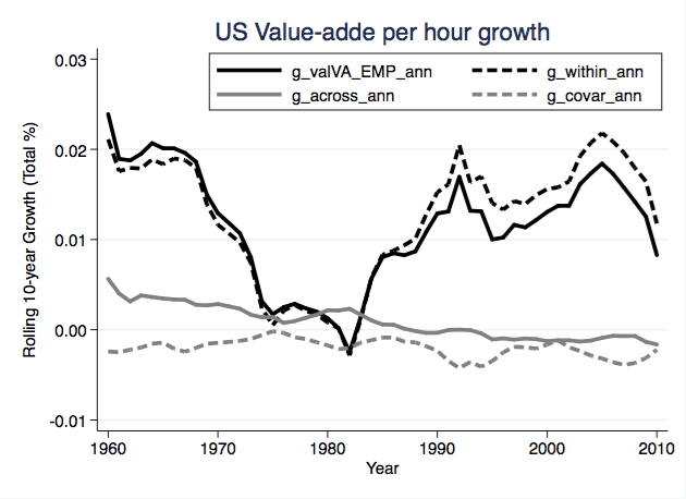
What is pretty clear is that within-sector growth is the dominant force in VAPH. And you can see the early high reported rates of growth of within-sector growth in the 1960’s (which capture growth from the 50’s into the 60’s). There is a clear slowdown in within sector growth from about 1975 to 1990, consistent with all the other evidence, and then things recover not quite back to the 1960’s level. The dip in 2009 and 2010 indicates that growth in VAPH from about 1999/2000 to 2009/2010 has been relatively slow, again consistent with our priors.
Now look at the contributions of across-sector growth and the covariance term. Across-sector growth is consistently positive throughout most of this period, but starts declining significantly around 1990, so that over the last ten years across-sector growth is negative for overall growth in VAPH. That means between 2000 and 2010 workers were moving out of sectors with high productivity (in 2000), and into sectors with low productivity (in 2000). Without any slowdown in actual productivity growth, measured aggregate productivity growth is going to be lower.
The negative contribution of the covariance term tells a similar story of negative effects, although this appears to be a consistent issue. Workers are not only moving into low productivity sectors to begin with, but into sectors with low productivity growth. This also drags down measured aggregate productivity growth.
The 10-year growth rate, starting in the 1990’s (which means the effects started in the early 80’s), no longer lies above the within-sector growth rate. In other words, starting in the 80’s, we see the across-sector and covariance effects of structural change producing a negligible or even negative effect on VAPH growth. This is most apparent in those final few years of the graph.
For Gordon’s critics, they can be right that individual technologies are still growing quickly, but what they do not account for is that labor may be moving out of those sectors and hence aggregrate growth could still be low. If we could get finer and finer levels of industry data, it is quite possible that what looks like a decline in within-sector growth in 2009/2010 is really just negative across-industry growth at those finer levels of industry. Gordon being wrong about whether specific technologies are improving does not make him wrong about aggregate growth declining.
At the same time, the fact that aggregate growth was high in the 40’s and 50’s doesn’t necessarily mean that individual technologies were improving faster than they are today.I don’t have the data, but I’d be fascinated to know what this figure looks like going backwards in the 1950’s and 1940’s, during Gordon’s golden age of productivity growth. Were those decades really a time of amazing “true” technological growth - which might be proxied by the within-sector effect - or did they benefit as much from strong across-sector and covariance terms?
One plausible reason for strong across-sector and covariance terms is the hump-shaped nature of demand for manufactured goods. In the 40’s and 50’s and 60’s, there was within-sector productivity growth in durable goods - refrigerators, TVs, cars - for sure. But this also generated large movements of people into those sectors, which would have produced big positive across-sector and covariance terms. Why? Because Americans didn’t own lots of refrigerators, cars, and TVs. Higher within-sector productivity would have lowered prices, and a high elasticity of demand would have meant those sectors pulled labor into those sectors.
But by the 70’s and later, higher within-sector productivity growth in durables and other manufatures may not have generated the same across-sector and covariance effects. Why? Because there are limits to durable good demand. Once everyone has a refrigerator, they tend to want to buy other things, and not another refrigerator. I know that’s not totally true; I have a 2nd fridge in my garage that serves as a strategic beer reserve. But in general, demand for durable goods becomes less elastic as we get richer. Which means that within-sector productivity gains don’t pull workers into manufacturing employment, it actively pushes them out. And because the sectors that labor is moving into are relatively low productivity, and have low productivity growth, we get negative across-sector and covariance terms. By the way, there is nothing here that William Baumol couldn’t have told you thirty years ago.
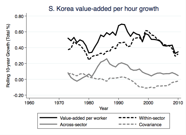
A comparison with South Korea is interesting, because they are several decades behind the US in this transformation. In the figure below I plotted the same rolling 10-year growth rates as for the US. It shows the big across-sector contribution to growth in South Korea in the 80’s and 90’s, as they were industrializing heavily and the elasticity of demand for those kinds of durable goods was still large. Compare the figures, and you’ll see that while the US may have had 8% total growth in VAPH due to across-sector effects at the maximum, in South Korea this maximum is closer to 40%. As South Korea got richer, this across-sector contribution has been falling, but is still adding about 6% to total growth in VAPH. The example of South Korea is why I think that part of the explanation for the rapid productivity growth in the US during the 40’s and 50’s could be across-sector effects, and not just a higher rate of innovation or technological change.
This has now gotten so long that I need to wrap it up. Let me try to do that by essentially repeating my summary from above. You cannot talk about aggregate productivity growth without talking about both technology and the distribution of workers across sectors. Anecdotes - positive or negative - about individual technologies are not informative about the aggregate level of productivity growth.