I told you I wouldn’t leave you waiting on the next post concerning markups and the paper by David Baqaee and Emmanuel Fahri, so here you go. In the last post, I described the (at times) paradoxical nature of markups. When there is dispersion in markups, output is lower than it could otherwise be, given technology. But when there is dispersion in markups, there are circumstances - like increasing markups in low-markup producers or shifting resources towards high-markup producers - where raising the average markup in the economy will be associated with higher output.
All that is in the BF paper, but it is not the main purpose of it. One of the main contributions of the paper is to show that you can generalize these effects of markups to almost any arbitrary model of the economy. The paradox is not just the result of making some particular assumptions about production functions or preferences.
One application they pursue (among many) is decomposing productivity growth into terms involving technology and terms involving allocative efficiency. If you read this blog at all, you know that productivity is a big bucket of different things going on in the economy. In that bucket are true technology effects, the ability to physically produce more widgets given some set of physical inputs. But also in that bucket are things like the allocation of those inputs across firms that produce different kinds of widgets.
Decomposing productivity growth
If the economy were perfectly efficient, meaning that the inputs we use were allocated across different firms such that we were at the maximum possible output level, then productivity would measure only true technological improvements. Yes, inputs might move between different firms in response to technological changes, but the efficiency of the economy is being held constant, and so those changes in input use have zero effect on productivity to a first approximation. The problem with using productivity to measure technology is not that inputs move around, per se, it is that the movement of inputs may not represent a move from one efficient equilibrium to another.
Let me give you an example to illustrate what I mean. Let’s say that in 2004, all the inputs (e.g. labor) in the economy were allocated in an efficient manner, and output was as high as it could possibly be given the specific physical technologies available in that year. We look at this allocation and say, clearly this is the best way to allocate inputs, so let’s pass a law to freeze the allocations at the 2004 shares. If 4% of all people worked at the Gap in 2004, then 4% of all people would always be required to work at the Gap.
In 2005, though, there are changes in the specific physical technologies used by different firms. Some may have better technology, some worse. Perhaps the Gap discovers a better way to fold shirts. Who knows. Because the technologies changed, there should be changes in the allocation of inputs. In an efficient economy, there would be changes in the allocations. But we have this dumb law that says the allocations cannot be changed.
From a productivity perspective, the growth in productivity - which remember is the output we can produce given a set of inputs - is affected by two things. First, there are the specific technological changes that occurred. By themselves, those should raise productivity (remember the cool new folding technique at the Gap). Second, there are now all the distortions introduced by the law. More than 4% of the labor force should work at the Gap now, but it is confined to only employing 4%. Thus we are getting less output than we could, and hence productivity is lower.
Productivity growth is thus a combination of the positive technological effect, and a negative effect of the allocation law. What we’d like to do is separate out those two effects. And that is what BF propose to do, in a setting that allows for any kind of arbitrary structure in terms of production functions, links between firms acting as suppliers to one another, and preferences. The contribution of their work is not to identify this issue in measuring productivity - we’ve known about that for a while - but to develop a way to manage that issue in almost any conceivable setting.
What do they do? Intuitively, they say you have to calculate the efficient outcome in 2005 given the changes in technology. Then you compare the productivity of this hypothetical efficient 2005 economy with the efficient 2004 economy, and in that case the productivity you measure is getting the “pure” effect of technology, holding constant the efficiency of the economy. In theory that is possible to do, but in practice it is hard (impossible) because you don’t know how much the true physical productivity of each firm improved over time. Hold on to that problem for a moment.
Once you’ve calculated this pure technological effect, you are left with changes in productivity that are due to changes in allocative efficiency. Here, the idea is that you are comparing the efficiency of the economy in 2004 to the efficiency of the economy in 2005, without asking about the technological changes. What BF show is that given some readily available data on markups and factor income shares (e.g. wages as a fraction of output) you can calculate this allocative efficiency effect without too much trouble, and this is true no matter how complex the underlying economy may be.
Overall productivity growth is thus a combination of the pure technology effect and the allocative efficiency effect. The simple math is
\[\% \Delta Prod = \% \Delta Tech + \% \Delta AE.\]BF have data on productivity growth (this is just the normal thing we calculate from data on output and inputs), and they show how to calculate $\% \Delta AE$. So in the end they don’t need to measure the precise technological changes of each firm, they can just back out the $\% \Delta Tech$ term from the above equation. You can infer the pure technological change in the economy once you measure the allocative efficiency change.
To implement this, BF need some way of measuring allocative efficiency, and they use the data on markups charged by firms. They draw this data from a paper from Gutierrez and Philippon that I talked about here. If you recall from the last post, markups push the economy away from the efficient allocation, and so BF can use changes in markups to measure the change in how far away from that efficient allocation the economy moves.
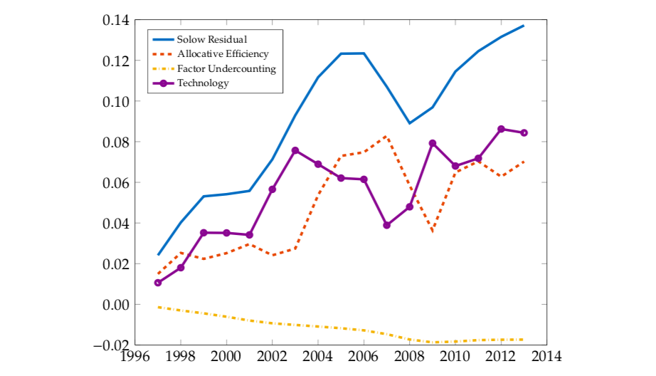
The results of all this are in the figure. The blue line, labelled the Solow residual, shows how productivity itself grows over time. This is what they are trying to decompose. The allocative efficiency line (orange dashes) is the contribution to productivity from changes in how close to the efficient allocation the economy got. Notice that this term is rising over time, meaning that according to their calculations the economy was more efficient in 2015 than in 1996. We’ll get back to that in a moment.
By definition, the difference between the blue line (productivity) and the orange dashed line (allocative efficiency) has to be the effect of pure technology. The purple line captures this, and you can see that this is also growing over time. But note that overall productivity grew faster than technology because of the allocative efficiency improvement. BF suggest that the each account for about 50% of the growth in productivity.
(You can also see one last source of growth in productivity, factor undercounting. I ignored this in my little analysis up above. This is capturing the fact that in the presence of markups the measure of inputs that we can calculate is not quite equal to the true level of input use. This effect can get very large - BF find it matters more using other data on markups that are larger than the Gutierrez and Philippon markups - but for the time being, lets set that effect aside.)
Wait, efficiency was going up?
The fact that BF find allocative efficiency was improving over time is perhaps surprising. To see why this was occurring, we can turn to a further decomposition that BF provide. To understand this, it helps to think of the allocative efficiency term as being determined by something like a weighted average of the markups across firms. As a weighted average, it can change over time for two reasons. The markups themselves could change, or the weights could change.
In the next figure, BF have separated out these two effects. The blue line is the same total allocative efficiency term from the first figure. The “markup effect” in orange dashes is measuring changes just the change in markups charged by firms, effectively holding the weights constant. The general increase in the “markup effect” comes from the fact that most markups were falling according to the Gutierrez and Philippon data. If you want to refer to the last post, this is telling us that all the markups in the economy were collapsing towards one (meaning no markup), and that the economy was getting closer to the point where the ratio of marginal utilites was equal to the ratio of marginal costs.
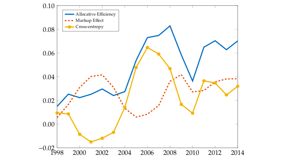
At the same time, we have what BF call the “cross-entropy” effect. That is not terribly informative. It refers to the fact that the weights in the weighted average of markups change over time. Recall that holding markups constant, if you push more resources into high-markup firms, this raises productivity because the output of those firms is very valuable. The yellow line shows that productivity was rising over time due to this effect, and that in turn implies that more and more resources were getting pushed into high markup firms.
The shift towards higher markup firms is consistent with the rise in profit share at the aggregate level. But that shift didn’t mean that productivity was falling. There are situations in which the rising profit share would be associated with lower productivity; if firm-specific markups were rising this would detract from productivity while raising profits. But what appears to have happened here is that profits rose due to changes in the composition of spending towards high-markup firms, and that is associated with higher productivity.
Revisiting Harberger’s triangle
The productivity accounting that BF do relates to changes in allocative efficiency, but only in a local sense. It tells us whether we are getting closer or farther from the efficient equilibrium, but it doesn’t tell us how far away the efficient equilibrium is to begin with. How much higher would output be if there were no markups?
BF use their setting to answer this question. The exact numbers depend on the precise set of markups they use, and some assumptions about the structure of the economy, but the answer is that output would be about 40% higher without markups. This is much, much, higher than the traditional answer, usually attributed to Harberger, who said the losses from monopoly were around 0.1%. Harberger’s number was always a bad estimate, as it was based on looking across sectors (not firms) only within manufacturing. It was an other example of assuming that what occurs within manufacturing is the only thing that matters. But even so, the scale of the effect that BF find is significant.
The big question is whether this substantial departure from the efficient equilibrium is worth it. We believe that markups are necessary to induce economic growth, as they provide the reward to those who innovate. Is operating 40% below the efficient outcome worth it, in the sense that the markups pushing us down there are in turn generating rapid growth? I have no idea what the answer to that question is. You’d need to build some more structure on top of the BF model to do that.
Here’s another interesting thing about their calculations, and it is an aspect of the paradox of markups. The 40% number BF calculate is for 2014. For 1997, they find that the loss associated with markups is only 4.5%. The loss associated with markups rose from 1997 to 2014, and yet allocative efficiency improved from 1997 to 2014, which is what the productivity calculations showed. How can those two things both be true?
BF’s productivity calculations show that the economy was moving towards the efficient equilibrium over time, and hence this contributed to productivity growth. But at the same time, the efficient equilibrium was moving farther and farther away. Think of me running a 100 meter race against Usain Bolt. He’s much faster, but I am running in the same direction, at least. My allocative efficiency improves, in the sense that I’m headed in the right direction. But my absolute efficiency declines, in the sense that Bolt gets farther and farther ahead of me every moment.
Again, without some more information, you can’t say whether falling further behind the efficient equilibrium is good or bad, but it is an interesting piece of information to throw into the mental wood chipper. It may be worth it to be further behind if that is associated with greater incentives to innovate. Or perhaps it is a correlate of the lack of dynamism in business formation and employment turnover that has been documented.
I have not even begun to scratch the surface of the interesting applications of the BF paper. I focused on the productivity accounting just because it is something I find to be of particular interest. The power of the paper is, to repeat, that these findings hold without having to make any strong assumptions about what production functions look like or how firms fit together into an input/output matrix. The only annoying thing about the paper is that it is forcing me to see how limited my understanding of the role of markups was in the economy. But it is well worth the effort to read it (so much notation!) if you’re into this kind of thing.