This is an odd post because it is an advertisement for a new paper that is …. in an advanced draft state? “Finished” is wrong because I’m about to embark on the roller-coaster that is submission and publication. But there are actual pages of text, and tables, and figures, and bibliography.
The paper itself is titled The Elasticity of Aggregate Output with Respect to Capital and Labor. Code and data for it can be found on Github.
If you’re a bit of a growth geek and somehow find that title intriguing, you can jump right to the link and read. Happy to receive comments. Otherwise, the rest of this post is an extended abstract explaining the main findings and how I got them.
Alpha equals what?
From a macro/policy perspective, it would be nice to know how sensitive GDP is to the stock of capital or the amount of labor used. Focusing on capital, I’d like to know the elasticity of GDP with respect to capital, or
\[\frac{d \ln Y}{d \ln K} = ??.\]Knowing that ?? number would inform me about things like the possible impact of a federal infrastructure bill, or the consequences of changes in savings behavior based on capital gains taxes, or the possible implications of demographic changes that influence home purchases and construction (capital goods). It’s got implications for how fast countries converge to steady state over time. It has a first-order effect on how we calculate TFP growth. It’s a relevant, important number, and you can make the same argument for why the elasticity of GDP with respect to labor is important.
Probably the most commonly used assumption in macro, and maybe in all of economics, is that this elasticity with respect to capital is equal to one-third. It’s even got it’s own greek letter. Hence you’ll see “alpha equals one-third” in a million macro papers, which refers to the coefficient $\alpha$ on capital in a Cobb-Douglas production function. If you’ve taken an intermediate macro course, you’ve seen this,
\[Y = K^{\alpha}(AL)^{1-\alpha},\]or something very, very close to it. If you take logs of this, you can figure out that $d \ln Y/ d \ln K = \alpha$.
That holds in general. Where does this idea that $\alpha = 1/3$ come from? That requires two big assumptions. First, it requires that there is such a thing as an aggregate production function. The existence of an aggregate production function requires a lot of underlying assumptions to be true. Felipe and McCombie refer to the aggregate production function as “not even wrong”, echoing Pauli’s assertion about a theory that was too incomplete to be used to make predictions. I think the best way to think about the issue is that an aggregate production function is pretending to be a statement about a physical relationship (e.g. combine two units of capital with three workers to get 12 widgets) as if it were a chemical formula. But because output is aggregate across goods using relative prices (and capital is handled similarly) the analogy just doesn’t hold.
Second, the rule of thumb about $\alpha = 1/3$ depends on the assumption that there are no economic profits in the economy. Without economic profits, it would be the case that $1-\alpha = wL/Y$ if the economy were cost-minimizing, with $wL$ being total labor compensation. Since we see that $wL/Y$ is about 2/3 in the data (or was until recently), that means $1-\alpha$ is about 2/3, and therefore $\alpha$ is about 1/3.
The common answer that “alpha equals on-third” delivers an answer to the question of what is the elasticity of GDP with respect to capital. But is it a meaningful answer, given that the assumptions it relies on are tenuous? It might be the right answer for a fictional economy that only exists on paper, but not in real life.
Higher, faster, farther
Can we do better? Yes. Thanks to recent work in a series of papers by David Baqaee and the late Emmanuel Farhi (see here and here for what I think are the right places to start) it is possible to break with the strict assumptions lying behind the aggregate Cobb-Douglas function and the rule of thumb “alpha equals one-third”.
In my paper, I’m taking their theory and calculating the elasticity $d \ln Y/ d \ln K$ (and a similar one for labor) while relaxing a bunch of the assumptions embedded in the rule of thumb. In particular, what do Baqaee and Farhi allow for?
-
Different units with different cost structures. In my case, the economy will have a bunch of different industries, each responding to capital and labor in a unique way. There is no need to assume that all industries have a similar Cobb-Douglas formula, or that it is Cobb-Douglas at all. Conceptually the theory could allow one to do this with information on all firms or establishments, I just don’t have that kind of detail.
-
Input-output relationships. Those industries can be suppliers to one another, as in real life. This means that the impact of some additional capital in one industry (e.g. a new truck) can have a cascade of effects on other industries by making their costs (e.g. of shipping) lower. The effect of capital on GDP depends on the network that connects these industries, and the aggregate elasticity I’m after is not just adding up the individual effects.
-
Frictions or markups. One of the big problems above was that it assumed zero economic profits, which a whole host of recent research (and baseline intuition) tells us is wrong. Each industry may be charging a markup of price over costs, and that could be due to market power or some other friction. The Baqaee/Farhi setting is flexible enough that the source of that markup doesn’t matter.
Baqaee/Farhi show how to find the aggregate elasticity I want from the industry-level information on costs of labor and capital. Before we move on, a couple of comments. First, this is like one tiny sliver of the Baqaee/Farhi theoretical setting. There are a ton of additional insights to work with. Second, my implementation of this is better than the rule of thumb, but it is not perfect. If you had data on each individual establishment and worker you could conceptually do this in an even more refined manner, improving on the numbers I’ll show you below.
Garbage in, garbage out
Okay, so I implement what Baqaee/Farhi came up with. Was that really that hard? Yes, because the data you need to stick into the formula that Baqaee/Farhi come up with is not immediately available from any national account. The core pieces of information you need are, for each industry, their cost of labor, their cost of intermediates purchased from other industries, and their cost of capital.
It’s this last one - the cost of capital - that creates the issue. The cost of capital is not reported in the national accounts, in large part because what we as economists consider the cost of capital is not what businesses think of when they talk about costs. Here’s one way to think about this.
When economists think of breaking down the value-added of an industry (it’s contribution to GDP) they do so in the following way
\[VA_i = COST_{iL} + COST_{iK} + EPROF_{i}\]or the value-added of industry $i$ gets accounted for by costs of labor (the first term), costs of capital (the second term), or economic profits (the last term). Those economic profits are often called “rents”, and refer to earnings the industry makes over and above the strict cost of production (labor and capital).
When businesses or the BEA breaks down value-added of an industry they do so more like this
\[VA_i = COST_{iL} + GOS_{i}\]where the cost of labor is the same, but the second term is “Gross Operating Surplus”. That gross operating surplus combines the cost of capital and the economic profits of the industry. Why? Think of an industry (or firm) who owns their capital outright (as opposed to renting it in). There is no “cost of capital” to record in the books. Everything that isn’t a cost of labor is an accounting profit for them, and the distinction between accounting profits they make due to owning capital versus earning economic profits is irrelevant.
But to do the Baqaee/Farhi calculation you have to have $COST_{iK}$. Gross operating surplus doesn’t cut it. So the game I play in my paper is coming up with various assumptions about how industries work to come up with estimates of $COST_{iK}$, and looking at what they imply for the elasticity of GDP with respect to capital.
I can’t come up with a single elasticity. I instead provide you, dear reader, with a set of bounds between which the real elasticity probably lives. What are the bounds?
-
No-profit upper bound. The first assumption is to assume that economic profits are zero. In that case you can see from the two prior equations that $COST_{iK} = GOS_i$, so this is measurable from the national accounts. But wait, isn’t this just what I said the rule of thumb did wrong? Yes! It was one of the assumptions in the rule of thumb. But even with this I’m still able to allow for the multiple industries and the input-output relationships, so this is a mild improvement over the rule of thumb. With this no-profit assumption note that the cost of capital is as large as it could be, and hence the elasticity of GDP with respect to capital is going to be as large as it could be. Thus this represents an upper bound.
-
Depreciation lower bound. The national accounts data don’t have a true cost of capital measure. But they have some information on costs of capital. In particular, they report the depreciation of capital for each industry, which is something like the minimal cost of capital that each industry faces - stuff breaks or wears out. Using depreciation to proxy for $COST_{iK}$, I can calculate the elasticity of GDP with respect to capital. Because this is like the minimal amount of capital cost each industry faces, it also represents the lower bound for the elasticity.
I could also bore you for a while with having to match industry-level data up bewteen the input-output tables and the national accounts, which is tedious and annoying and I hated it and it took by far the most time in all of this. But none of you want to hear about that.
What do I find? The figure below shows you the core result. The dashed line on top is the estimated elasticity of GDP with respect to capital when I use the no-profit assumption described, and the solid line on the bottom is the elasticity using the depreciation cost assumption. The real elasticity lives somewhere in that gray zone in between them. Note this isn’t a confidence interval, and there is nothing telling us that the real elasticity must be in the middle.
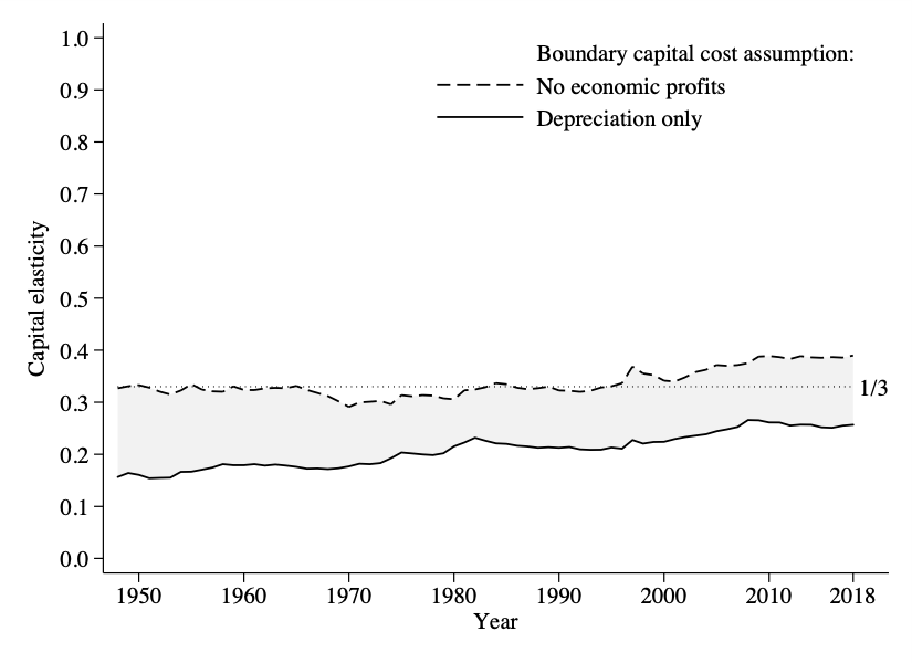
Note that for most of this period the elasticity lies below one-third, or the rule of thumb is probably over-stating how sensitive GDP is to capital. That possible changed around 1998, when the bounds both start to drift up. It doesn’t prove the actual elasticity changed, but starts to imply it. The rule of thumb isn’t exactly right, and it probably makes sense to think of this elasticity being lower than one-third, but not by a lot.
Incidentally, the labor elasticity is just the reverse of this, as the labor elasticity is going to be one minus the capital elasticity. So turn your phone upside down and look at the figure and you’ll get the bounds for the labor elasticity.
There are a lot of variations one can run with this, and that is a lot of what the paper does. One version that I find interesting is to consider the elasticity of private business sector output with respect to capital. The private business sector is GDP minus housing and the government. The next figure shows you the same kinds of bounds (no-profit and depreciation) for this more limited slice of the economy.
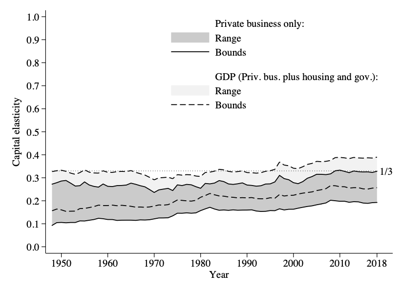
The range is shifted down by about 0.05 or so everywhere. That means the private business sector is less sensitive to capital than the economy as a whole. Why? Mainly because housing value-added is very, very, sensitive to capital. Remember, the BEA imputes the value-added from housing as the rents that you would pay yourself for living in your home. That imputed rent almost all ends up being attributed as a capital cost rather than a labor cost. A big reason that one-third is even plausible as an upper bound for the elasticity is because housing is extremely sensitive to capital. Absent that, the economy appears to be less sensitive as a whole.
Um, so who cares?
One of the things that this elasticity gets used for is in backing out TFP growth. The standard way to calculate TFP growth is as follows
\[d \ln TFP_t = d \ln Y_t - \epsilon_K d \ln K_t - \epsilon_L d \ln L_t\]which shows that TFP growth is just what is “left over” after you subtract off the growth of capital and labor from the growth in GDP. The weights on the growth rate of capital and labor are the elasticities, $\epsilon_K$ and $\epsilon_L$. These elasticities are what I was calculating above, and I’m just using the greek letters here as shorthand.
If you go to the BLS and look at their TFP growth estimates, they infer $\epsilon_K$ and $\epsilon_L$ using a similar rule of thumb to $\alpha = 1/3$. They don’t assume that $\epsilon_K$ is literally fixed for all time, but they do assume that they can back out the value of $\epsilon_L$ and $\epsilon_K$ using the no-profit assumption. That means they are using the highest possible estimate for $\epsilon_K$, and the lowest possible one for $\epsilon_L$. But we know this is an extreme assumption, so it may well be over or understating TFP growth.
What do you get if you use different estimates of $\epsilon_K$ and $\epsilon_L$, based on the Baqaee/Farhi calculations I do? Then this changes the implied growth rate of TFP, and hence the implied path of TFP over time.
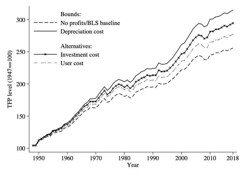
In this figure, the lowest line matches what the BLS calculates for the level of TFP over time (starting from a baseline of 100 in 1948). The other lines show the implied path of TFP when you use different estimates of $\epsilon_K$ and $\epsilon_L$ depending on the assumptions about capital costs. The top solid line is when you use depreciation costs to measure capital costs, and the implied elasticity on capital is lower (and the elasticity on labor is higher). TFP ends up higher by about 20% (a little over 300 versus about 250 in 2018). The intermediate cases are based on some other assumptions about capital costs that lead to different estimates of $\epsilon_K$ and $\epsilon_L$.
Nothing about this changes the general picture of TFP growth over time. There’s a slowdown in the 1970s into the 1980s. There is more rapid growth in the late 1990s. There is another slowdown in the 21st century. But the implied growth rate the BLS gets is almost certainly a lower bound to actual TFP growth. Which means the level of TFP is higher today than the BLS would imply, and that the trend growth rate is slightly higher than they would tell you.
I think there are a number of other applications of these elasticities. The Baqaee/Farhi setting gives you the ability to talk about a very complex production side of the economy (I/O relationships, multiple industries, markups) in a very concise way. These elasticities give you the sensitivity of the aggregate economy to capital and labor with all those complications already embedded in them. It means you can answer questions about policy, demographics, and TFP for an economy with all those complications, but without having to model all those complications explicitly. The elasticities are sufficient for a lot of purposes.
As I said above, this is not definitive. One could drill down even further and come up with even more refined estimates of those elasticities. But it is an improvement on the rule of thumb, and gives some sense of how that rule of thumb likely overshoots the right elasticity with respect to capital (and undershoots it with respect to labor).